Reduced Graph Powers

For a monomeric receptor model with state-transition diagram \(G\), the state-transition diagram for the homodimer (assuming identical subunits) is the reduced graph power \(G^{(2)}\). This expanded state-transition diagram for the receptor dimer can be created in Sagemath by constructing the Cartesian product \(G \Box G\) by merging vertices that are equivalent up to symmetry.

To illustrate, consider a receptor model with topology given by the path graph \(P_4\).

P4 = graphs.PathGraph(5)
P4.show(figsize=2)

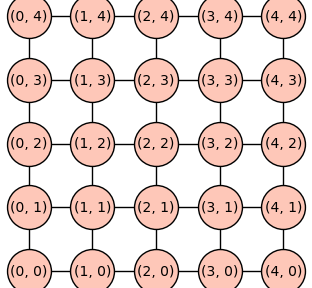
The Cartesian product \(P_4 \Box P_4\) can be constructed using the Sagemath method cartesian_product.

P4P4 = P4.cartesian_product(P4)
pos = {v: v for v in P4P4.vertices(sort=True)}
P4P4.set_pos(pos)
P4P4.show(figsize=4,vertex_size=1000)

The function cartesian_power below takes a graph \(G\) and integer \(k\) as input and constructs the Cartesian power graph \(G \Box G \Box \cdots \Box G\) with \(k\) fators. The \(k\)-the Cartesian power graph is denoted \(G^k\).

def cartesian_power(G=Graph(), k=2):
    # Make Cartesian power G^k (unreduced)
    Gk=G.copy()
    for i in range(k-1):
        Gk = Gk.cartesian_product(G)
    # Make each vertex a tuple
    vflat=list(range(Gk.order()));
    for i in range(Gk.order()):
        v=Gk.vertices(sort=True)[i]
        vflat[i]=tuple(flatten(v))
    Gk.relabel(vflat)
    return Gk

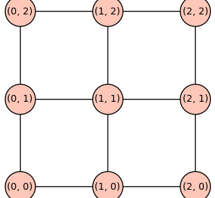
P3P3 = cartesian_power(graphs.PathGraph(3))
pos = {v: v for v in P3P3.vertices(sort=True)}
P3P3.set_pos(pos)
P3P3.show(figsize=4,vertex_size=1000)

P3P3P3 = cartesian_power(graphs.PathGraph(3),3)
P3P3P3.show3d()

The following code block constructs the Cartesian product graph \(G \Box G\) (GG) and then merges vertices that are equivalent by symmetry. The result is the reduced graph power \(G^{(2)}\) (G2).

def reduced_cartesian_power(G=Graph(), k=2):
    Gk = cartesian_power(G, k)
    for v in Gk.vertices(sort=True):
        for u in Gk.vertices(sort=True):
            sv=tuple(sorted(v))
            su=tuple(sorted(u))
            if v!=u and sv==su and v<u and Gk.has_vertex(v) and Gk.has_vertex(u):
                Gk.merge_vertices([v,u])
    return Gk

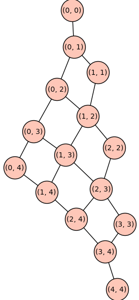
To illustrate we construct the reduced Cartesian power \(P_4^{2}\).

P42 = reduced_cartesian_power(P4)
P42.show(figsize=8,vertex_size=1000)

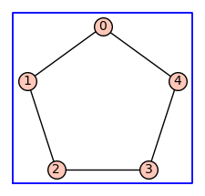
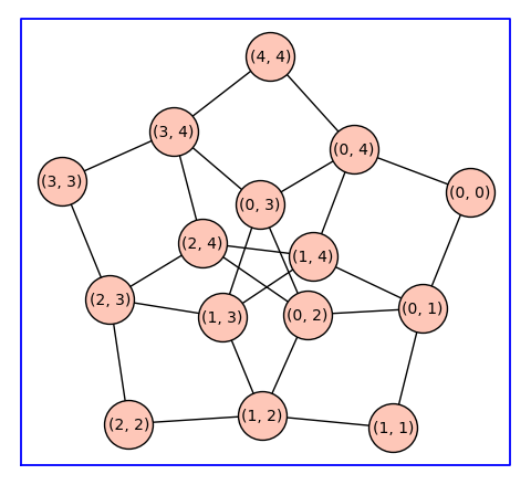
Below we construct the cycle graph \(C_5\), the Cartesian product graph \(C_5 \Box C_5\), and the reduced Cartesian power \(C_5^(2)\).

C5 = graphs.CycleGraph(5)
C5.show(figsize=3,graph_border=True)
C52 = reduced_cartesian_power(C5)
C52.show(figsize=6,vertex_size=1000,graph_border=True)

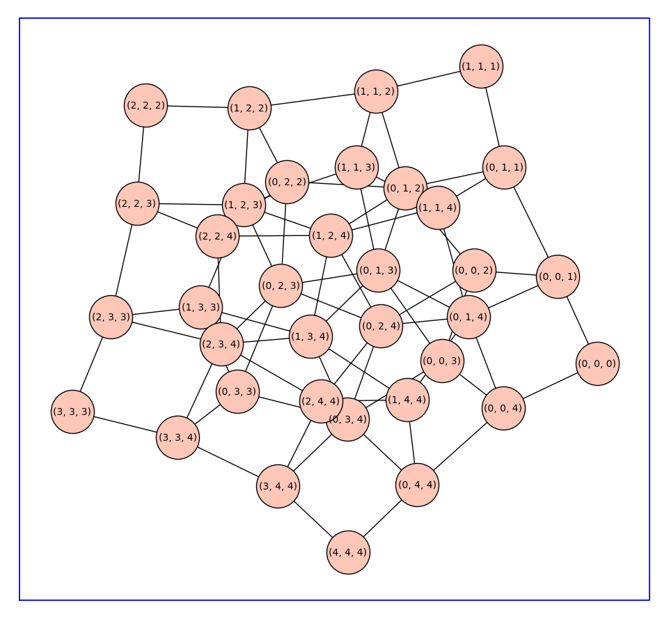
Beginning with a monomer model with state-transition diagram \(G\), the state-transition diagram for a receptor \(k\)-mer is given by reduced Cartesian power \(G^(k)\). Below we constuct \(C_5^3\).

C53 = reduced_cartesian_power(C5,3)
C53.show(figsize=12,vertex_size=2000,graph_border=True)

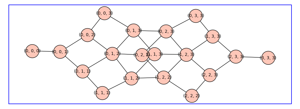
Below is the reduced Cartesian power \(P_4^3\).

P43 = reduced_cartesian_power(graphs.PathGraph(4),3)
P43.show(figsize=10,vertex_size=1000,graph_border=True)
P43.show3d()

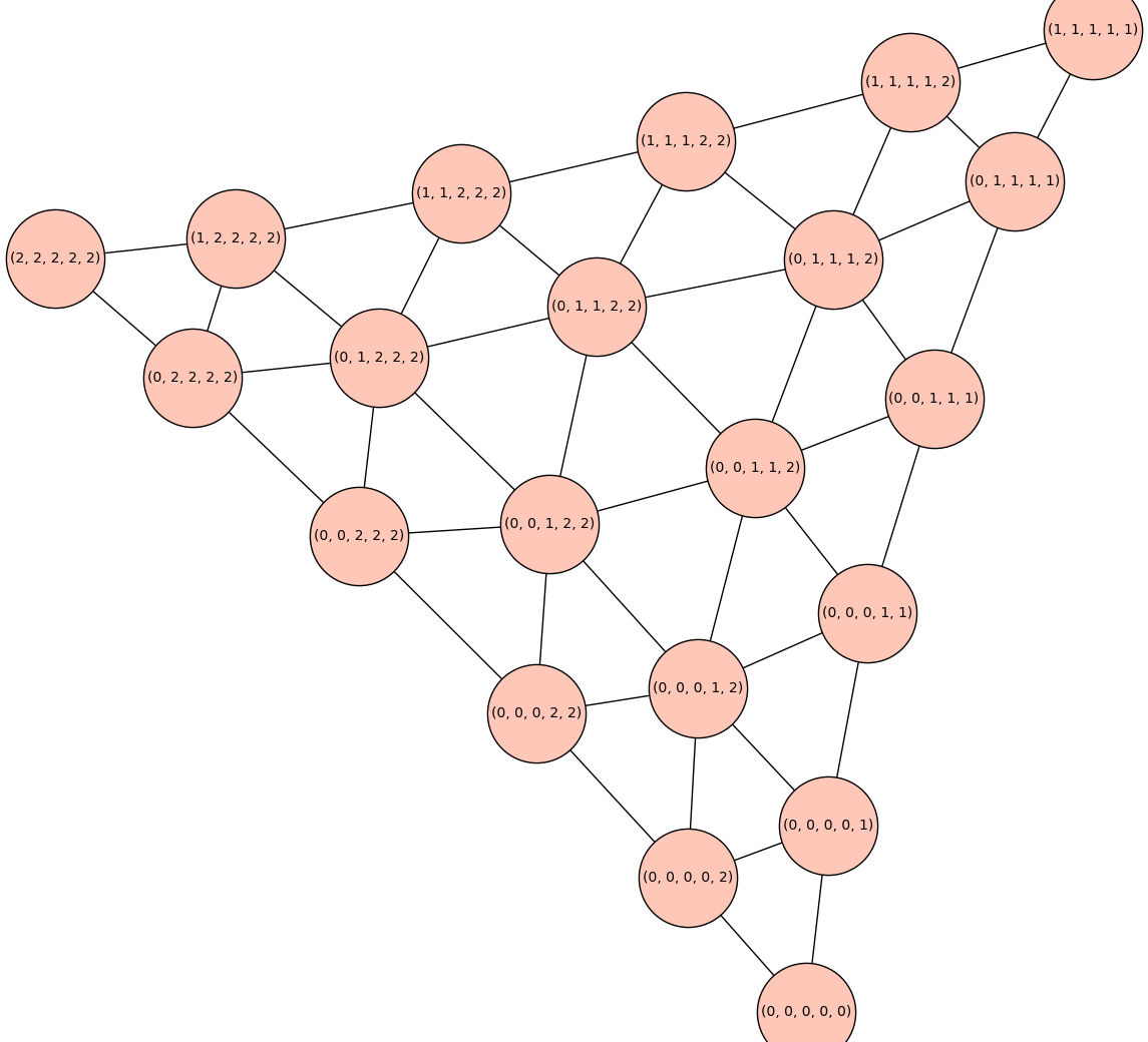
The reduced Cartesian power \(C_3^k\) has the structure of a triangular lattice. For example, \(C_3^5\) is show below.

C3_5 = reduced_cartesian_power(graphs.CycleGraph(3),5)
C3_5.show(figsize=14,vertex_size=5000)

For more information about reduced graph products, see

• Richard H. Hammack and Gregory D. Smith, Cycle bases of reduced powers of graphs, ARS Mathematica Contemporanea, 12(1):183–203, 2017. doi: 10.26493/1855-3974.856.4d2