Using MyTools.ipynb - Part 2 - Enumerating allosteric parameters in receptor dimers#
This notebook illustrates some of the function definitions contained in MyTools.ipynb.
The file MyTools.ipynb includes the function enumerate_allosteric_parameters(G) which takes a graph G and returns the \(\kappa\) and \(\eta\) values for a dimer model with the topology of the reduced graph power \(G^{(2)}\). The default method uses \(e_1, e_2, \ldots , e_v\) while method='alpha' gives single digit edge labels (\(b,c,\ldots\)).
%run MyTools.ipynb
mydoc(myfun, method='both')
Display the signature of myfun followed by the docstring of myfun.
Set method ='signature' or 'method = 'docstring' or 'method = 'both'
my_graph_show(G)
Show a graph Greg’s way.
Prints the vertices and edges of the graph G.
add_vertex_monomials(G=Graph on 0 vertices, method='integer', ring=False)
Add monomials to vertices of a graph.
The add_vertex_monomials function takes a graph G, as well as optional parameters method and ring. The function creates a new graph H with vertices labeled by monomials. The monomials are chosen based on the number of vertices in G. If the method parameter is set to ‘alpha’ and the number of vertices in G is less than or equal to 10, the monomials are chosen as alphabetical letters (‘a’ to ‘k’). Otherwise, the monomials are chosen as strings of the form ‘a0’, ‘a1’, …, ‘an-1’, where n is the number of vertices in G. The function then adds the vertices from G to H using the monomials as labels, and adds the edges from G to H using the monomials as endpoints. If the ring parameter is set to True, the function also creates a polynomial ring V with the chosen monomials and ‘invlex’ order, and returns both H and V. Otherwise, it returns only H.
INPUT:
G– graph object (default:Graph());method– integer (default:integer);
OUTPUT: The graph with monomials as vertices
EXAMPLES:
This example illustrates … ::
sage: A = ModuliSpace()
sage: A.point(2,3)
xxx
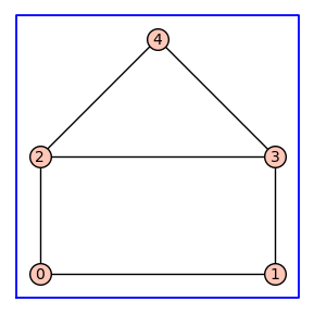
Below we will consider a receptor model with the topology of the house graph. Note that G=graph.HouseGraph() constructs a graph G with integer vertices.
G=graphs.HouseGraph()
G.show(figsize=4,graph_border=True)
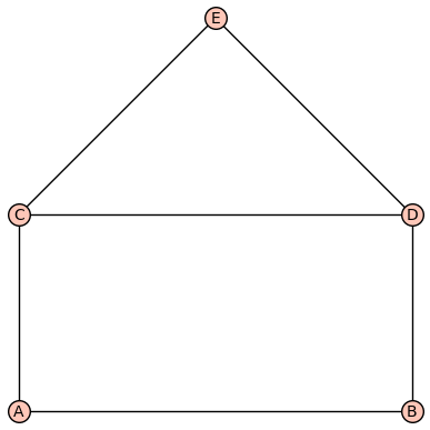
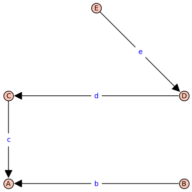
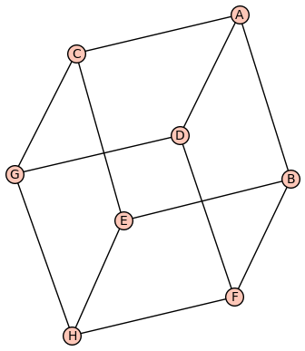
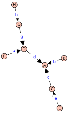
The method = alpha has replaces the vertices with monomials. The spanning tree is constructed with BFS labeling. KappaEta is a list of lists giving the probability of each state as a symbolic expression which is displayed in LaTeX format. The polynomial ring A has the \(\kappa_i\) and \(\eta_{ij}\) as symbolic variables for \(0 \leq i,j \leq v-1\).
(G, T, KappaEta, A) = enumerate_allosteric_parameters(G,method='alpha',show=True)
| \(1\) | \(2 \kappa_{\mathit{b}}\) | \(2 \kappa_{\mathit{c}}\) | \(2 \kappa_{\mathit{c}} \kappa_{\mathit{d}}\) | \(2 \kappa_{\mathit{c}} \kappa_{\mathit{d}} \kappa_{\mathit{e}}\) |
| \(0\) | \(\kappa_{\mathit{b}}^{2} \eta_{\mathit{bb}}\) | \(2 \kappa_{\mathit{b}} \kappa_{\mathit{c}} \eta_{\mathit{bc}}\) | \(2 \kappa_{\mathit{b}} \kappa_{\mathit{c}} \kappa_{\mathit{d}} \eta_{\mathit{bc}} \eta_{\mathit{bd}}\) | \(2 \kappa_{\mathit{b}} \kappa_{\mathit{c}} \kappa_{\mathit{d}} \kappa_{\mathit{e}} \eta_{\mathit{bc}} \eta_{\mathit{bd}} \eta_{\mathit{be}}\) |
| \(0\) | \(0\) | \(\kappa_{\mathit{c}}^{2} \eta_{\mathit{cc}}\) | \(2 \kappa_{\mathit{c}}^{2} \kappa_{\mathit{d}} \eta_{\mathit{cc}} \eta_{\mathit{cd}}\) | \(2 \kappa_{\mathit{c}}^{2} \kappa_{\mathit{d}} \kappa_{\mathit{e}} \eta_{\mathit{cc}} \eta_{\mathit{cd}} \eta_{\mathit{ce}}\) |
| \(0\) | \(0\) | \(0\) | \(\kappa_{\mathit{c}}^{2} \kappa_{\mathit{d}}^{2} \eta_{\mathit{cc}} \eta_{\mathit{cd}}^{2} \eta_{\mathit{dd}}\) | \(2 \kappa_{\mathit{c}}^{2} \kappa_{\mathit{d}}^{2} \kappa_{\mathit{e}} \eta_{\mathit{cc}} \eta_{\mathit{cd}}^{2} \eta_{\mathit{dd}} \eta_{\mathit{ce}} \eta_{\mathit{de}}\) |
| \(0\) | \(0\) | \(0\) | \(0\) | \(\kappa_{\mathit{c}}^{2} \kappa_{\mathit{d}}^{2} \kappa_{\mathit{e}}^{2} \eta_{\mathit{cc}} \eta_{\mathit{cd}}^{2} \eta_{\mathit{dd}} \eta_{\mathit{ce}}^{2} \eta_{\mathit{de}}^{2} \eta_{\mathit{ee}}\) |
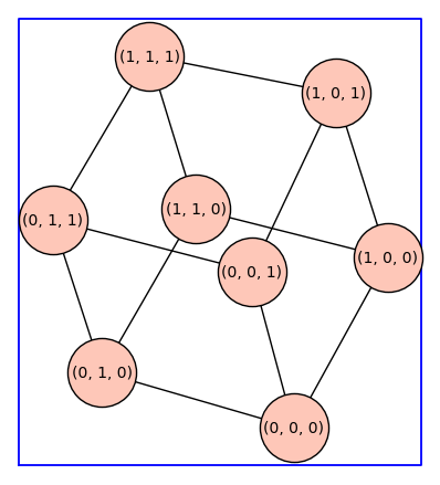
The next example is reminicent of the cubic ternary complex model. Note that graphs.GridGraph([2,2,2]) has tuples as vertices. We use cannonical_label() to make the vertices integers. This is necessary because enumerate_allosteric_parameters() requires a graph G with integer vertices.
G=graphs.GridGraph([2,2,2])
G.show(figsize=6,graph_border=True,vertex_size=2000)
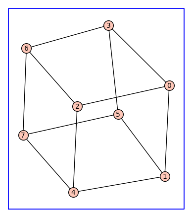
G=G.canonical_label()
G.show(figsize=6,graph_border=True)
(G, T, KappaEta, A) = enumerate_allosteric_parameters(G,method='alpha',show=True)
| \(1\) | \(2 \kappa_{\mathit{b}}\) | \(2 \kappa_{\mathit{c}}\) | \(2 \kappa_{\mathit{d}}\) | \(2 \kappa_{\mathit{c}} \kappa_{\mathit{e}}\) | \(2 \kappa_{\mathit{d}} \kappa_{\mathit{f}}\) | \(2 \kappa_{\mathit{d}} \kappa_{\mathit{g}}\) | \(2 \kappa_{\mathit{d}} \kappa_{\mathit{g}} \kappa_{\mathit{h}}\) |
| \(0\) | \(\kappa_{\mathit{b}}^{2} \eta_{\mathit{bb}}\) | \(2 \kappa_{\mathit{b}} \kappa_{\mathit{c}} \eta_{\mathit{bc}}\) | \(2 \kappa_{\mathit{b}} \kappa_{\mathit{d}} \eta_{\mathit{bd}}\) | \(2 \kappa_{\mathit{b}} \kappa_{\mathit{c}} \kappa_{\mathit{e}} \eta_{\mathit{bc}} \eta_{\mathit{be}}\) | \(2 \kappa_{\mathit{b}} \kappa_{\mathit{d}} \kappa_{\mathit{f}} \eta_{\mathit{bd}} \eta_{\mathit{bf}}\) | \(2 \kappa_{\mathit{b}} \kappa_{\mathit{d}} \kappa_{\mathit{g}} \eta_{\mathit{bd}} \eta_{\mathit{bg}}\) | \(2 \kappa_{\mathit{b}} \kappa_{\mathit{d}} \kappa_{\mathit{g}} \kappa_{\mathit{h}} \eta_{\mathit{bd}} \eta_{\mathit{bg}} \eta_{\mathit{bh}}\) |
| \(0\) | \(0\) | \(\kappa_{\mathit{c}}^{2} \eta_{\mathit{cc}}\) | \(2 \kappa_{\mathit{c}} \kappa_{\mathit{d}} \eta_{\mathit{cd}}\) | \(2 \kappa_{\mathit{c}}^{2} \kappa_{\mathit{e}} \eta_{\mathit{cc}} \eta_{\mathit{ce}}\) | \(2 \kappa_{\mathit{c}} \kappa_{\mathit{d}} \kappa_{\mathit{f}} \eta_{\mathit{cd}} \eta_{\mathit{cf}}\) | \(2 \kappa_{\mathit{c}} \kappa_{\mathit{d}} \kappa_{\mathit{g}} \eta_{\mathit{cd}} \eta_{\mathit{cg}}\) | \(2 \kappa_{\mathit{c}} \kappa_{\mathit{d}} \kappa_{\mathit{g}} \kappa_{\mathit{h}} \eta_{\mathit{cd}} \eta_{\mathit{cg}} \eta_{\mathit{ch}}\) |
| \(0\) | \(0\) | \(0\) | \(\kappa_{\mathit{d}}^{2} \eta_{\mathit{dd}}\) | \(2 \kappa_{\mathit{c}} \kappa_{\mathit{d}} \kappa_{\mathit{e}} \eta_{\mathit{cd}} \eta_{\mathit{de}}\) | \(2 \kappa_{\mathit{d}}^{2} \kappa_{\mathit{f}} \eta_{\mathit{dd}} \eta_{\mathit{df}}\) | \(2 \kappa_{\mathit{d}}^{2} \kappa_{\mathit{g}} \eta_{\mathit{dd}} \eta_{\mathit{dg}}\) | \(2 \kappa_{\mathit{d}}^{2} \kappa_{\mathit{g}} \kappa_{\mathit{h}} \eta_{\mathit{dd}} \eta_{\mathit{dg}} \eta_{\mathit{dh}}\) |
| \(0\) | \(0\) | \(0\) | \(0\) | \(\kappa_{\mathit{c}}^{2} \kappa_{\mathit{e}}^{2} \eta_{\mathit{cc}} \eta_{\mathit{ce}}^{2} \eta_{\mathit{ee}}\) | \(2 \kappa_{\mathit{c}} \kappa_{\mathit{d}} \kappa_{\mathit{e}} \kappa_{\mathit{f}} \eta_{\mathit{cd}} \eta_{\mathit{de}} \eta_{\mathit{cf}} \eta_{\mathit{ef}}\) | \(2 \kappa_{\mathit{c}} \kappa_{\mathit{d}} \kappa_{\mathit{e}} \kappa_{\mathit{g}} \eta_{\mathit{cd}} \eta_{\mathit{de}} \eta_{\mathit{cg}} \eta_{\mathit{eg}}\) | \(2 \kappa_{\mathit{c}} \kappa_{\mathit{d}} \kappa_{\mathit{e}} \kappa_{\mathit{g}} \kappa_{\mathit{h}} \eta_{\mathit{cd}} \eta_{\mathit{de}} \eta_{\mathit{cg}} \eta_{\mathit{eg}} \eta_{\mathit{ch}} \eta_{\mathit{eh}}\) |
| \(0\) | \(0\) | \(0\) | \(0\) | \(0\) | \(\kappa_{\mathit{d}}^{2} \kappa_{\mathit{f}}^{2} \eta_{\mathit{dd}} \eta_{\mathit{df}}^{2} \eta_{\mathit{ff}}\) | \(2 \kappa_{\mathit{d}}^{2} \kappa_{\mathit{f}} \kappa_{\mathit{g}} \eta_{\mathit{dd}} \eta_{\mathit{df}} \eta_{\mathit{dg}} \eta_{\mathit{fg}}\) | \(2 \kappa_{\mathit{d}}^{2} \kappa_{\mathit{f}} \kappa_{\mathit{g}} \kappa_{\mathit{h}} \eta_{\mathit{dd}} \eta_{\mathit{df}} \eta_{\mathit{dg}} \eta_{\mathit{fg}} \eta_{\mathit{dh}} \eta_{\mathit{fh}}\) |
| \(0\) | \(0\) | \(0\) | \(0\) | \(0\) | \(0\) | \(\kappa_{\mathit{d}}^{2} \kappa_{\mathit{g}}^{2} \eta_{\mathit{dd}} \eta_{\mathit{dg}}^{2} \eta_{\mathit{gg}}\) | \(2 \kappa_{\mathit{d}}^{2} \kappa_{\mathit{g}}^{2} \kappa_{\mathit{h}} \eta_{\mathit{dd}} \eta_{\mathit{dg}}^{2} \eta_{\mathit{gg}} \eta_{\mathit{dh}} \eta_{\mathit{gh}}\) |
| \(0\) | \(0\) | \(0\) | \(0\) | \(0\) | \(0\) | \(0\) | \(\kappa_{\mathit{d}}^{2} \kappa_{\mathit{g}}^{2} \kappa_{\mathit{h}}^{2} \eta_{\mathit{dd}} \eta_{\mathit{dg}}^{2} \eta_{\mathit{gg}} \eta_{\mathit{dh}}^{2} \eta_{\mathit{gh}}^{2} \eta_{\mathit{hh}}\) |
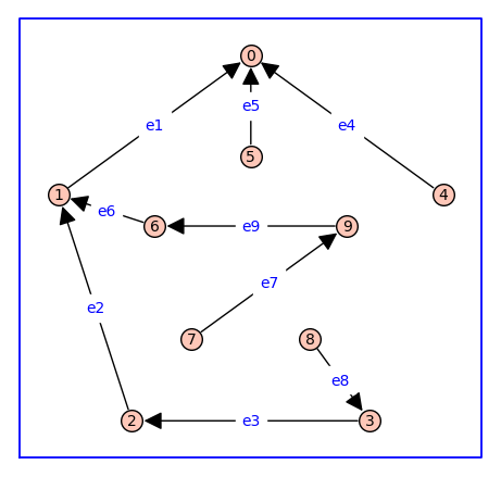
An example of a receptor model with more states. Using show=False suppresses the output. One can still work with the ring A, show the BFS spanning tree, and list the probability of each state.
(G, T, KappaEta, A) = enumerate_allosteric_parameters(graphs.PetersenGraph(),method='integer',show=False)
A.inject_variables()
Defining kappa_1, kappa_2, kappa_3, kappa_4, kappa_5, kappa_6, kappa_7, kappa_8, kappa_9, eta_11, eta_12, eta_22, eta_13, eta_23, eta_33, eta_14, eta_24, eta_34, eta_44, eta_15, eta_25, eta_35, eta_45, eta_55, eta_16, eta_26, eta_36, eta_46, eta_56, eta_66, eta_17, eta_27, eta_37, eta_47, eta_57, eta_67, eta_77, eta_18, eta_28, eta_38, eta_48, eta_58, eta_68, eta_78, eta_88, eta_19, eta_29, eta_39, eta_49, eta_59, eta_69, eta_79, eta_89, eta_99
T.show(figsize=6,graph_border=True,edge_labels=True)
from IPython.display import display, Math
for i,k in enumerate(flatten(KappaEta)):
    if k != 0:
        display(Math(latex(i)+':'+latex(k)))