Receptor modeling - scraps#
var('a12, a21, a13, a31, a23, a32, a34, a43')
d = {1: {2:a12, 3:a13}, 2: {1:a21, 3:a23}, 3: {2:a32, 1:a31, 4:a34}, 4: {3:a43}};
G = DiGraph(d,weighted=True)
G.plot(figsize=8,edge_labels=True,pos=vertex_positions,graph_border=True)
---------------------------------------------------------------------------
NameError                                 Traceback (most recent call last)
Cell In[1], line 4
      2 d = {Integer(1): {Integer(2):a12, Integer(3):a13}, Integer(2): {Integer(1):a21, Integer(3):a23}, Integer(3): {Integer(2):a32, Integer(1):a31, Integer(4):a34}, Integer(4): {Integer(3):a43}};
      3 G = DiGraph(d,weighted=True)
----> 4 G.plot(figsize=Integer(8),edge_labels=True,pos=vertex_positions,graph_border=True)

NameError: name 'vertex_positions' is not defined
The weighted adjacency matrix for G is
A = G.weighted_adjacency_matrix()
A
[  0 a12 a13   0]
[a21   0 a23   0]
[a31 a32   0 a34]
[  0   0 a43   0]
The Laplacian of G is:
L = G.laplacian_matrix()
L
[      a21 + a31            -a12            -a13               0]
[           -a21       a12 + a32            -a23               0]
[           -a31            -a32 a13 + a23 + a43            -a34]
[              0               0            -a43             a34]
This matrix is sometimes referred to as the combinatorial Laplacian matrix of the weighted directed graph G.
Generator matrix and Laplacian#
The generator matrix Q for the Markov chain associated to G can be constructed from the weighted adjacency matrix A as folows.
Q = A - diagonal_matrix(sum(A.T))
The following code defines e to be column vector of ones. This is used to show that each row of Q sums to zero.
e = matrix([1,1,1,1]).T
print(Q*e)
[0]
[0]
[0]
[0]
Multiplying on the left by the transpose of e, given by e.T, we see that each column of Q does not sum to zero.
print(e.T*Q)
[ -a12 - a13 + a21 + a31 a12 - a21 - a23 + a32 a13 + a23 - a31 - a32 - a34 + a43 a34 - a43]
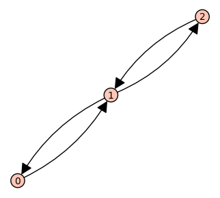
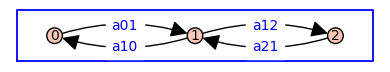
Three state model#
As a simple example, consider a receptor model with three states arranged as follows.
G = DiGraph({0: {1:'a01'}, 1: {0:'a10', 2:'a12'}, 2: {1:'a21'}})
pos = {0: (0, 0), 1: (1, 0), 2: (2, 0)}
G.plot(figsize=4,edge_labels=True,pos=pos,graph_border=True)
G = DiGraph({'R': {'RL':'kap*L'}, 'RL': {'R':'kam', 'RLL':'kbp*L'}, 'RLL': {'RL':'kbm'}})
pos = {'R': (0, 0), 'RL': (1, 0), 'RLL': (2, 0)}
G.plot(figsize=4,edge_labels=True,pos=pos,graph_border=True,vertex_size=1000)
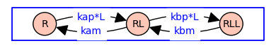
When both forward and reverse transitions are explicit, the state-transition diagram has the topology of a symmetric directed version of the path graph with 3 vertices.
Here is the (undirected) path graph \(P_3\):
G = Graph({0: [1], 1: [2]})
G.plot(figsize=4)
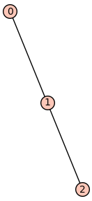
The symmetric directed version is